Chapter 7Real data as splats
A splat is a number-carrying blob: a place, three sizes, a turn, a color, an opacity. Data
is also numbers with places: the atoms of a protein, the quakes of last week, the stars over
your head, the density of a scanned walnut. This chapter is about turning such data into
splats, and doing it honestly: every Splash here says where its data came from and how old
it is. Nearly all of these Splashes are behind the labs switch (add ?labs=1 to
the site's address); the paragraphs say which.
Molecules
What it is. A molecule is a list of atoms with places, in ångströms. The
Molecule Viewer opens a structure file and draws it as splats. It reads PDB, mmCIF,
SDF/MOL, and XYZ files (src/molview/parse.js), takes the first model, and stops
with a message above 250,000 atoms. You can open a file from your device, or type a
four-character Protein Data Bank code and have the viewer fetch that entry. It draws balls
and sticks, space-filling atoms, a cartoon of the chains as ribbons, or the molecular
surface, and colors by element, chain, residue, B-factor (how much an atom blurs in the
crystal), position along a chain, or secondary structure. Tap two atoms for the distance
between them, a third for the angle. It is behind the labs switch.
How Splashery does it. Everything is an explicit splat
(src/molview/draw.js): an atom is a sphere of splats (in space-filling style,
one of its van der Waals radius), a bond is a stick of splats (a double bond is two thinner
sticks, a triple bond three), the cartoon is a ribbon of splats along a path through the
backbone, and the surface is a blobby surface made from a sum of bumps, one per atom. The
device's splat budget decides how many splats there are. A small molecule gets plenty per
atom. A big structure gets fewer, and below about six splats an atom becomes one round
Gaussian, so even a big structure opens on a phone: that is the level of detail (Chapter 2).
The files are read in a worker, off the page's main thread, and the structure is turned so
its widest spread lies across the screen. A turn keeps every distance and angle.
The PDB fetch. Typing a code asks files.rcsb.org for that one file
(public, no key, no account), only when you press the button. Nothing is sent but the code
in the address, nothing is stored, and the file is read on your device. The viewer refuses a
file over 60 MB. Five samples ship with the site, so the Splash opens offline: crambin, the
green fluorescent protein, lysozyme, a stretch of B-DNA, and caffeine; each is a snapshot of
the entry, dated October 5, 2026, and the data are CC0 from the Protein Data Bank [14].
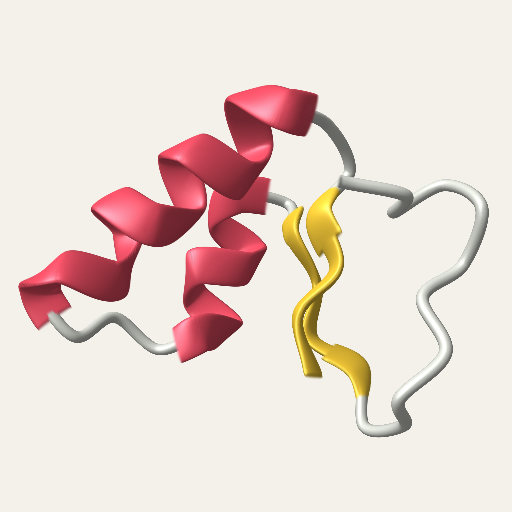
The Molecule Viewer's cartoon
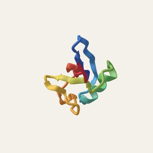
The Protein Splash, on the Atoms shelf
The rest of the Atoms shelf. Beyond the molecules, the shelf has the Atom, Electron Orbital, and the Periodic Table, which are open to everyone, and, behind the labs switch, Unit Cells (crystal structures from the Crystallography Open Database, CC0), Orbital Atlas, and Real Elements (a photo of each element, credited beside it). The Periodic Table's lettering (the atomic numbers, the symbols, and the row markers) is the same at every splat count from Mid up, and changing the Element keeps the board and builds only the atom and its frames again. Unit Cells and Electron Orbital open farther out, at 5.2 of their radii, so a phone shows the whole block of cells and the whole orbital.
Try it. Molecule Viewer (labs), Protein, Molecule.
Earthquakes
What it is. A globe with a dot for every earthquake in a feed from the U.S. Geological Survey, drawn on a relief of the Earth. A bigger quake is a bigger dot. The color says how deep the quake was: shallow ones orange-red, middle ones yellow and green, and the deepest blue, as the USGS's own maps do. The globe is the Earth in true color with its relief. A tap plays the quakes in time order, each flashing as the timeline passes it.
How Splashery does it. The Splash offers three views: the past week at magnitude 2.5 and up, the past month at 4.5 and up, and a year at 5 and up. The first two read the USGS's GeoJSON summary feeds [15] when the Splash opens or when you tap its plaque to refresh. Each quake is a row of five numbers (time, longitude, latitude, depth in kilometers, magnitude). A quake with a missing magnitude or depth is left out rather than shown as zero. A dot's radius is 0.009 + 0.006 × (M − 2)1.4 times the globe's radius (for a magnitude of 2 or more), drawn as a flat disc of splats with a crisp edge, and a bigger dot gets more splats, in proportion to its area. The plaque beside the globe says what is showing: the feed, the number of quakes, and when it was made. If the feed cannot be reached within 9 seconds, or if the browser is being driven by a test tool, the Splash shows the snapshot that ships with the site (197 quakes in the week view as of October 5, 2026, 14:39 UTC), and the plaque says "snapshot". The year view is always a snapshot, October 2025 to September 2026.
Why this way. Splashery has no server, so a live feed has to be read by your browser from a public, keyless address, and it has to degrade: an offline reader still gets a globe. The week and month feeds come from the USGS, so your browser asks the USGS directly, with no Splashery server between them. The USGS receives that request as it would from any visitor to its own site: your IP address, your browser's usual headers, and Splashery's address as the page that asked. The year view and the snapshot send no request. The rules for every such Splash are in the box at the end of this chapter.
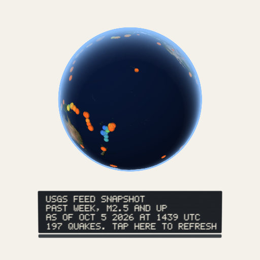
Try it. Earthquakes (labs).
The Night Sky
What it is. The stars and planets above a place, for any date and time and any place. You stand at the center of the dome and look out; the Sun, the Moon, and the seven planets are placed from the date (the planets' tables are made for 1800 to 2050, and the Splash says so when you go outside them), the Moon is lit on the side that faces the Sun (so its phase is the real geometry), and daylight washes the stars out faintest first.
How Splashery does it. The sky, the ground, the stars, the Moon, the Sun, and the planets are drawn with the stage's textured meshes, not splats. Only the constellation lines, the ring a tap draws, and the compass letters are splats. The sky dome works out the light scattered once at each of its vertices, for the Sun and for the Moon (by air, by haze, and by ozone, with the Earth's shadow), and adds twilight's light scattered more than once, an airglow that brightens toward the horizon, and the Milky Way from the European Space Agency's Gaia map. The stars are the HYG database [16] to magnitude 6, plus 20,720 fainter HYG stars from magnitude 6.0 to 7.5. Each is a sharp point, a Gaussian core 0.45 pixels wide with a faint halo, whose light follows its magnitude and whose color follows its B−V index (how blue or red it is), dimmed and reddened by the air it shines through. The planets are points by magnitude. The Moon is NASA's LROC map, lit from the Sun's side, and the Sun is a disc; both are drawn at their real size but never smaller than 12 and 8 pixels across, so in a wide view they are larger than life (the Splash's About says so). One exposure follows the brightness of the zenith part of the way, so stars come out in twilight brightest first and fade under a bright Moon.
The stars sit at their J2000 positions, and the whole sky turns as one rigid piece: first precession to the date, then the sky's turn for the place's sidereal time (Meeus [17]). The planets use the approximate orbital elements that NASA's Jet Propulsion Laboratory publishes for 1800 to 2050 [18], solved with Kepler's equation, and the Moon uses the Astronomical Almanac's low-precision series, good to about 0.3 degrees in longitude. The constellation lines, which are splats, are a part that the same turn moves: the same hinge as every part in Chapter 2, a star field turning about its pivot.
Tapping and zooming. A tap names the star, planet, Moon, or Sun that shows within 24 pixels of your finger, the brightest first, and a tap with none near clears the name. On a phone the legend lets a tap through to the sky, so a star under it can be named. A pinch narrows the view to 3 degrees, where a finger's width is about 6 arcminutes and close pairs such as Mizar and Alcor (12 arcminutes apart) come apart.
Your place. You pick a city, or tap Use my location, which asks your browser for it. That is the only time the Splash asks. The place lives in the page's memory: it is not saved, not put in a link, and not sent anywhere. Both the stars and the constellation lines come from sources under CC BY-SA 4.0, and the Splash's credit says so beside it. The Milky Way is ESA/Gaia/DPAC's map (CC BY-SA 3.0 IGO) and the Moon's is NASA's (public domain); both are credited beside the Splash too.
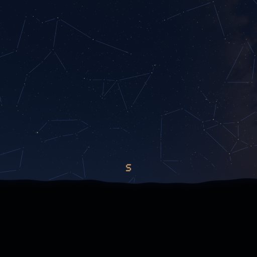
Try it. Night Sky (labs).
Space: the real worlds
What it is. The Space shelf has two kinds of world. The real ones are globes built from real elevation and imagery: Real Earth, Real Moon, Real Mars, Real Mercury, Real Venus, Real Moons (Io, Europa, Ganymede, Callisto, and Titan), and Small Worlds (Pluto, Ceres, and Vesta). The planets named Model (Solar Model, Mercury Model, Venus Model, Earth Model, Moon Model, and Mars Model) are built in the page and are open to everyone; the real worlds are behind the labs switch. A tap on Moon Model lands a lunar module, and an astronaut plants a flag; its Flag option, in the Splash sheet, picks which flag.
How Splashery does it. Each real world is made from public-domain data, credited beside it: Real Earth from NASA's Blue Marble and NOAA's ETOPO 2022 relief (with NASA's Black Marble night lights and Natural Earth's place names), Real Moon from NASA's lunar color mosaic and elevation, Real Mars from the Viking color mosaic and the MOLA elevation, Real Mercury from the MESSENGER mission, Real Venus from Magellan, and Real Moons and Small Worlds from the Galileo, Voyager, Cassini, New Horizons, and Dawn missions. Their place names come from the International Astronomical Union's gazetteer. A tap turns the spot under your finger to the middle, builds a dense patch of splats there, and glides in (Everest, Machu Picchu, Fuji, and Kilimanjaro are examples on Real Earth); a tap while you are zoomed in goes back out. A Relief option lifts the ground from 5 to 40 times, or leaves it at its true height.
The zoom. A tap's zoom starts as its turn ends. If the dense patch is not built yet, the zoom glides in on the globe on show, slowing to a stop 40% of its way in, and the patch takes over at the frame it lands. A zoom moves at most a 30 Hz frame's worth from one frame to the next, so a frame that runs long holds the picture a moment instead of leaping ahead. A zoom tapped back out stops building its patch.
Labels and place names. A place is labeled only while it faces the camera, by more than 0.12 (the cosine of its angle from the view), so labels hide near the limb. A label that would cross another moves to its dot's other side or shows its dot alone, and the labels that face the camera most are placed first. Labels sit on their places from a link or an embed as well. The place names load once the world is shown, in the page's idle time after its first frame (a second at most), or at the first tap if that comes sooner; a tap before they are in names its place once they come, and its zoom waits for them.
Three more Space Splashes use real data. In Star Explorer, a tap zooms in to the named star nearest the spot (65 stars have names) and stays, with the star ringed and named with its distance; the next tap goes back out, and Play visits the brightest in turn. Its data are the Gaia Catalogue of Nearby Stars (ESA/Gaia/DPAC, CC BY-SA 3.0 IGO) and the HYG database (CC BY-SA 4.0). In Powers of Ten, the Zoom slider scrubs the journey while it plays or is paused: a drag, a pinch, or the wheel takes over, and the journey stops where it is. Its pictures come from several sources under several licenses, each credited beside it. Solar System puts the planets on their real orbits from JPL's tables and names its bodies in a sharp 12-pixel layer over the stage.
Try it. Real Earth, Real Moon, Star Explorer, Powers of Ten, and Solar System (all labs).
Volumes and point clouds
What it is. A CT scan or an MRI is not a surface but a block of numbers, one per little cube (a voxel), measuring how dense the material is there. A lidar scan is a cloud of points with places and sometimes colors. Both can be splats. The Volume Viewer opens a medical or microscope scan and shows it as a block of splats you can cut through. The Point Clouds Splash opens a lidar scan or any list of points. Both are on the Studio shelf, behind the labs switch, and nothing is uploaded.
How Splashery does it: volumes. The viewer reads DICOM (a series of slices, a folder,
a zip, or one multi-frame file; uncompressed or RLE lossless), NIfTI (.nii and
.nii.gz), TIFF stacks, and raw files described by a small form
(src/volume/read.js). Slices are sorted by where the scanner put them, and the
spacing between slices comes from those places, so a scan that is thick in one direction
keeps its true shape. A volume is at most 8 million voxels in memory; a bigger one is
averaged down as it is read, so the density grid it keeps is never more than about 32 MB (16
MB on a phone-sized device). Reading the file and drawing the splats use more memory
besides. The splats sit on a lattice spaced to fit the device's budget. A density
window (a lower and an upper level) decides which values show; the presets are bone,
soft tissue, and full range, and for a CT in Hounsfield units bone is 300 to 1500 and soft
tissue is −160 to 240. A color map turns the value into a color and an opacity. A cutting
plane on each axis, which a drag moves, hides the splats on one side. A
maximum-intensity view flattens the volume to the brightest voxel along one axis.
Splashery's engine has a splat kind for this (volume): each splat carries its
density, the shader tests it against the window, and the cut is tested at the splat's place
at rest, so the cut stays with the specimen as it turns.
How Splashery does it: point clouds. The Splash opens LAS, LAZ, PLY, XYZ, and PTS files (LAZ through the vendored laz-perf decoder, loaded only for a LAZ file). The points are drawn as splats within the device's budget, colored by height, by intensity, by classification (ground, vegetation, buildings, and the other codes a lidar file uses), or by the file's own colors. You can measure between two taps, crop, thin the cloud, and save it as PLY, LAS, or XYZ. The three samples are lidar from the U.S. Geological Survey's 3D Elevation Program, public domain: the Palace of Fine Arts and Fort Point in San Francisco, and Meteor Crater in Arizona, each thinned to 450,000 points.
The Imaging shelf. Walnut CT sits on its own shelf, Imaging, ready to cut through. The shelf also has five Splashes built in the page about how a scanner or a camera sees, all behind the labs switch: CT Explained, Airport X-ray, Fruit MRI, Electron Microscope, and Thermal Camera. In Fruit MRI, a drag on the fruit moves the slice the way the Slice slider does: right or up moves it on, and left or down moves it back.
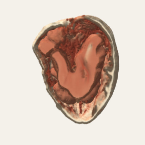
A CT scan of a walnut
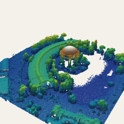
Lidar, colored by height
Why this way. A splat can stand for a voxel or a point without any new idea: it is a place, a size, and a color. What the Splash has to add is a way to look inside, and that is the window and the cutting plane. Rendering a volume with splats gives up the smooth shading of a proper volume renderer, in return for the same engine, the same controls, and a saved link that opens it in the same viewer as everything else.
Try it. Volume Viewer, Walnut CT, Point Clouds (all labs).
Weather, maps, and the other data Splashes
Most of the data Splashes ship a dated snapshot that a tool on a build machine fetched once, so the page itself never calls a data service. The Splashes are:
- Hurricane (labs): Hurricane Polo, September 21 and 22, 2026. GOES infrared cloud tops over a satellite map of the Earth, with the eyewall and bands turning. A tap plays the day it grew from 70 to 155 knots, following the storm's best track.
- Bar Harbor Tides (labs): a coastal height map and imagery of the harbor in Maine, with NOAA's tide predictions for a spring tide; a tap plays the day and the sandbar to Bar Island floods and dries.
- Grand Canyon, Mount St. Helens, and The Sea Floor (labs): heights from the USGS 3D Elevation Program and NOAA's ETOPO1 relief, as terrain made of splats.
-
Stork Migration
(labs): 30 white storks tagged in Germany, flying their real GPS tracks to Africa in fall
2013 (Movebank, CC0). The track file ships with the site; the tool that downloaded it is
in
tools/. - Climate Records (labs): NOAA's Mauna Loa carbon dioxide record as a rising spiral, one turn a year, and NASA's temperature anomalies as a field of monthly bars or a wall of yearly stripes. Dated snapshots, never fetched live.
- 3D Data (labs): open a CSV or TSV from your device, pick the columns for X, Y, Z, color, and size, and see a scatter, bars, or a surface with labeled axes that turn to face you. Three small sample tables ship with it. It saves a picture (PNG) or a turning video (WebM) to a file you choose.
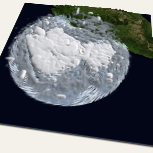
Hurricane Polo
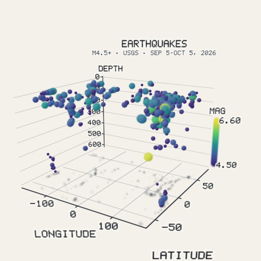
3D Data: the quakes as a scatter
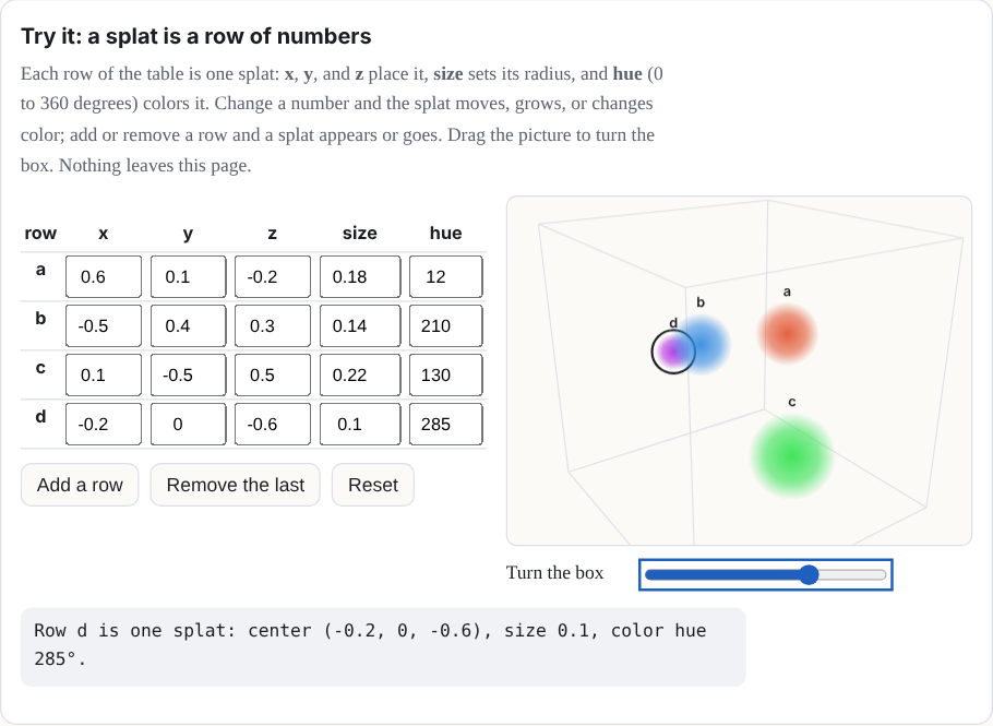
Try it: a splat is a row of numbers
Each row of the table is one splat: x, y, and z place it, size sets its radius, and hue (0 to 360 degrees) colors it. Change a number and the splat moves, grows, or changes color; add or remove a row and a splat appears or goes. Drag the picture to turn the box. Nothing leaves this page.
| row | x | y | z | size | hue |
|---|
The rules for live data
A Splash that reads from outside the page follows a short list of rules:
- Only a public endpoint that needs no key or account, and only data, never code: the earthquake feed, an entry from the Protein Data Bank. (Other open feeds, such as animal tracking, may be read the same way when their terms allow; today the stork tracks ship as a file.)
- It happens when you open the Splash or tap to refresh, never before.
- The source and the time of the data show beside it.
- Nothing is stored and nothing is sent, except the request for the data itself.
- A dated snapshot ships with the site, for when the feed cannot be reached.
- The Night Sky may ask for your location, only when you tap for it, and never stores or sends it.
A Wikipedia book, which would fetch an article when the reader asks for it (CC BY-SA text, never stored or shipped), is planned. The rules allow it, but it is not built yet, so it is not in this manual's list of Splashes.
Where to try it
- Protein and Molecule (always on); Molecule Viewer (labs).
- Earthquakes, Night Sky, Volume Viewer, Point Clouds, Hurricane, and 3D Data (all labs).
- Real Earth, Star Explorer, and Powers of Ten: real worlds and real stars (all labs).
- Fruit MRI, CT Explained, Unit Cells, and Real Elements (all labs).